
Quantitative Susceptibility Mapping (QSM) provides a map of local tissue magnetic susceptibility. QSM is a novel contrast mechanism in MRI compared to traditional hypointensity contrast in SWI or T2* weighted images that only allow detection of the presence of tissue susceptibility. Hypointensity reflects effects of regional, not local tissue susceptibility and is contaminated by blooming artifacts that vary with image parameters. QSM overcomes these problems by utilizing both magnitude and phase data and performing a dipole deconvolution. QSM enables quantitative investigation of local tissue susceptibility property. QSM is useful for identification and quantification of specific biomarkers including iron, calcium, gadolinium, and super paramagnetic iron oxide (SPIO) nano-particles.
MATLAB implementations and validation on testing datasets are available here
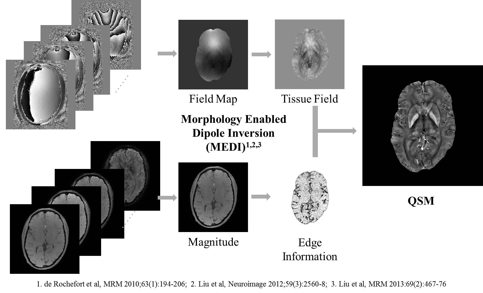
An outline of the MEDI QSM reconstruction. Typical QSM scan time is 7 minutes at 3T.
MEDI Toolbox is a collection of MATLAB routines for reconstructing the Quantitative Susceptibility Map (QSM) using the Morphology Enabled Dipole Inversion (MEDI) method. This toolbox also includes background field removal methods, such as Projection onto Dipole Fields (PDF) and Laplacian Boundary Value (LBV).
To download the Toolbox and sample data, register here . The download link will be provided on the confirmation page.
The code has been tested on 64 bits Windows 7 MATLAB R2009a, Mac OSX 10.8 MATLAB R2013a and Ubuntu 10.04 MATLAB R2009a.
We welcome all potential collaborators in our ongoing research. We are interested in a wide variety of applications for quantitative susceptibility mapping (QSM) in both human and animal imaging. If you are interested in collaborating with us, these are a few suggestions on the imaging parameters for your subject and data format that would greatly facilitate data processing.
The following parameters have been tested on GE scanners to generate satisfactory image results, and is extendable to Philips and Siemens scanners. (Essential parameters are underlined).
Use a 3D multi-echo gradient echo sequence with flow compensation. The real & imaginary images or magnitude & phase images need to be saved in DICOM format. Parallel imaging can be turned on to reduce scan time as long as the required images can be properly reconstructed.
Other parameters are as follows:
The following parameters have been tested on Bruker scanners to quantify SPIO on the order of 30ng. The detection limit is roughly proportional to 1/(SNR*TElast*B0). Please feel free to adjust the parameters accordingly. (Essential parameters are underlined).
Use a 3D multi-echo gradient echo sequence with flow compensation. True orthogonal planes are recommended. For Bruker scans, raw data (fid) and imaging parameters (acqp) are welcome. Otherwise, the real & imaginary images or magnitude & phase images need to be saved in DICOM format.
Other parameters are as follows:
Some general QSM information can be found on the QSM Wikipedia Page as well as at QSMMRI.com.
For further information, please contact Dr. Yi Wang (yiwang@med.cornell.edu). We are constantly optimizing these parameters. Please let us know if these protocols do not currently meet your need. We will be glad to study the situation with you and improve the acquisition.